LCA CIFAR Tutorial
This version of the tutorial is deprecated. The current version of the tutorial begins with Part 1.
This tutorial will walk you through implementing our modified LCA algorithm in OpenPV. You will learn a dictionary from the CIFAR dataset and run analysis code on the output of the simulation.
This tutorial assumes you have OpenPV and all dependencies downloaded and built with the CUDA, cuDNN, and OpenMP flags on. For further information on installation, please refer to:
All files referenced from this tutorial are available on the repository.
The topics of this tutorial will cover
- 1. A quick overview of the algorithm
- 2. Setting up the run via parameter files
- 3. Learning a set of basis vectors from the CIFAR dataset
- 4. Analysis of the output

Natural scenes can be decomposed into basic image primitives using sparse coding (Olshausen, Field, 1996). A patch of an image can be represented as a weighted (T(u)) linear sum of a set of feature vectors (ɸ). There exists an infinite number of ways to reconstruct the image patch. However, sparse coding restricts the network by limiting the number of feature vectors that can be used to reconstruct this patch. The sparse coding energy function describes a tradeoff between the number of active elements and reconstruction fidelity, controlled by a free parameter λ. Minimizing the energy function with respect to ɸ generates a code that creates a faithful reconstruction of the image using as few feature vectors as possible. These feature vectors (ɸ) can be learned using a Hebbian weight update rule. For images of natural scenes, these feature vectors are Gabor-like edge detector filters or shading elements (in the case of non-whitened inputs).
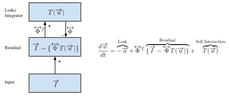
The Locally Competitive Algorithm (LCA) (Rozell et al., 2008) is a dynamical sparse solver. The big advantage of such a model is that all computations are local, allowing for the algorithm to be massively parallelizable. Here, the residual is the difference between the input and the reconstruction. This in turn drives the thresholded activations u, changing the reconstruction to better explain the input. These dynamics converge to create a sparse representation of the input. Updates to ɸ are done via a Hebbian learning rule between the residual and the V1 layers.
This tutorial uses /path/to/source/OpenPV as the path to the OpenPV source directory, and /path/to/build-OpenPV as the path to the build directory. Replace these paths as necessary with those for your system.
First, navigate to the build directory. Then copy the directory LCA-CIFAR-Tutorial from the source directory, and switch into it.
$ cd /path/to/build-OpenPV
$ cp -r /path/to/source/OpenPV/tutorials/LCA-CIFAR LCA-CIFAR-Tutorial
$ cd LCA-CIFAR-Tutorial
The LCA-CIFAR-Tutorial directory contains the directories scripts and input.
Then, get the CIFAR dataset from the CIFAR website, or enter the following commands in terminal to get the dataset.
$ wget "http://www.cs.toronto.edu/~kriz/cifar-10-matlab.tar.gz"
$ tar -zxvf cifar-10-matlab.tar.gz
The script extractCIFAR will extract the CIFAR images from the MATLAB .mat files.
$ cd scripts
$ octave extractCIFAR.m
$ cd ../
If you do not have octave, you can also extract the images using python3. The python script depends on the imageio and scipy packages.
$ python scripts/extractCIFAR.pyextractCIFAR takes several minutes. It creates folders named by each dataset, all the images in each
dataset, and corresponding text files listing all the image paths each dataset. Finally, the script concatenates all of the image paths into a file called mixed_cifar.txt.
The full parameter file for our CIFAR run is a Lua script in the input directory; it can be found here. The most relevant parameters of the model are set at the top, with documentation on what each parameter does. Change various paths as necessary. The rest of these parameters are already tuned for this tutorial.
To find PetaVision-specific Lua modules, the Lua script reads the
environment variable PV_SOURCEDIR for the OpenPV source directory. If this
variable is not set, it uses $HOME/OpenPV as the default.
Set PV_SOURCEDIR to your PV source directory, and then run the Lua script to generate a .params file, which will be used as input to the PetaVision binary:
$ export PV_SOURCEDIR=/path/to/source/OpenPV
$ lua input/LCA_CIFAR_full.lua > input/LCA_Cifar.params
To view the block diagram of the parameter file, run the draw tool.
$PV_SOURCEDIR/python/draw -l -p input/LCA_Cifar.paramsThe visualization of the parameter file should look like so.

-
Inputtakes images from 'mixed_cifar.txt', normalizes luminance, and passes its values toInputErroron the positive channel, where the values are simply copied over. -
InputErrorcomputes the difference between the input and the reconstruction fromInputRecon, which drives the minimization of the sparse coding energy function inV1. - The connection from
V1toInputErroris a plastic connection that uses a Hebbian learning rule to update weights in the direction of the gradient.
Lua allows for some abstraction of an OpenPV params file. The generated parameter file is verbose, and contains:
- one column (a container for the network where network-level parameters are specified)
- layers (Perform computations)
- connections (Communicate information and perform transformations between layers)
- probes (Record and save variables from the cost function - energy, reconstruction error, sparsity, etc. Used to calculate the adaptive time step) This section is optional, and goes into details of various parameters of the generated parameter file.
The column is the outermost wrapper of the simulation; all the layers are proportional to the column. The column sets up a bunch of key simulation details such as how long to run, where to save files, how frequently and where to checkpoint, and adaptive time-step parameters. Here are a few of the important ones:
| HyPerCol Parameter | Description |
|---|---|
startTime |
sets where experiment starts; usually 0 |
stopTime |
sets how long to run experiment; (start - stop)/dt = number of timesteps |
dt |
length of timestep; modulations possible with adaptive timestep |
outputPath |
sets directory path for experiment output |
nx |
x-dimensions of column; typically match to input image size |
ny |
y-dimensions of column; typically match to input image size |
checkpointWriteDir |
sets directory path for experiment checkpoints; usually output/Checkpoints |
dtAdaptFlag |
tells OpenPV to use the adaptive timestep parameters for normalized error layers |
For more details on the HyPerCol please read the documentation: HyPerCol Parameters
The layers are where the neurons are contained and their dynamics described. You can set up layers that convolve inputs, have self-self interactions, or even just copy the layer properties or activities of one layer to another and more. All layers are subclassed from HyPerLayer and you can read about their individual properties by following some of the Doxygen documentation.
Some important parameters to notice are nxScale, nyScale and nf since they set up physical dimensions of the layer. phase and displayPeriod describe some of the temporal dynamics of the layer. Most layers have their own unique properties that you can explore further on your own. For now this is a good snapshot. The table below summarizes the types of layers we use and roles in this experiment:
| Layer Class | "Name" | Description |
|---|---|---|
ImageLayer |
"Input" |
loads images from inputPath |
HyPerLayer |
"InputError" |
computes residual error between Input and V1 |
HyPerLCALayer |
"V1" |
codes a sparse representation of Input using LCA |
HyPerLayer |
"InputRecon" |
reconstruction of input, feeds back into error |
Let's look more closely at some more of the layer parameters: displayPeriod, writeStep, triggerFlag, and phase. ImageLayer has a parameter 'displayPeriod' that sets the number of timesteps an image is shown. We then typically set the writeStep and initialWriteTime to be some integer interval of displayPeriod, but this isn't necessary. For example if you want to see what the sparse reconstruction looks like while the same image is being shown to V1, you can change the writeStep for "InputRecon" to 1 (just note that your output file will get very large very quickly so you may want change the stopTime to a smaller value if you want this sort of visualization).
writeStep determines how frequently OpenPV outputs to the .pvp file (this is the unique binary format used for OpenPV). Triggering can be used to specify when a layer or connection will perform updates. The default behavior is to update every time step. For example, the MomentumConn V1ToInputError has triggerLayerName = "Input". This means that the connection will only update its weights when Input presents a new image.
Normally, we would like to view the reconstruction after converging on a sparse approximation. This is where phase comes in. Phase determines the order of layers to update at a given timestep. In this tutorial, the phases are fairly straightforward, however there might be cases when a different behavior is desired.
| Layer Class | "Name" | Phase |
|---|---|---|
ImageLayer |
"Input" |
0 |
HyPerLayer |
"InputError" |
1 |
HyPerLCALayer |
"V1" |
2 |
HyPerLayer |
"InputRecon" |
3 |
For more details on the HyPerLayer parameters please read the documentation: HyPerLayer Parameters
The connections connect neurons to other neurons in different layers. Similar to layers, connections are all subclassed from their base class HyPerConn. Connections can learn weights, transform, and scale data from one layer to another.
Connections in OpenPV are always described in terms of their pre and postLayerName, their channel code, and their patch size (or receptive field). We use a naming convention of [PreLayerName]To[PostLayerName] but it is not required if you explicitly define the pre and post layer.
The channelCode value determines if the connection is excitatory (0), inhibitory (1), or passive (-1). In a typical ANN layer, we subtract the input of the inhibitory channel from the excitatory channel. Passive does not actually deliver any data to the post layer, but is useful when you want a connection to only learn weights.
Patch size is determined by the nxp, nyp, and nfp parameters. Restrictions on how you can set these values are explained in detail in [Patch Size and Margin Width Requirements].
The following table summarizes the types of connections that are used and their roles in this experiment:
| Connection Class | "Name" | Description |
|---|---|---|
RescaleConn |
"InputToError" |
Copies and scales the input to the error layer |
TransposeConn |
"ErrorToV1" |
Transposes (flips pre/post) the V1ToError weights |
MomentumConn |
"V1ToError" |
A learning connection that uses a momentum learning rate |
CloneConn |
"V1ToRecon" |
Clones V1toError weights to send to reconstruction |
IdentConn |
"ReconToError" |
Copies the reconstruction activities to the error layers negative channel |
For more details on the HyPerConn parameters please read the documentation: HyPerConn Parameters
Probes are used to calculate the energy of the network and adapt the timescale used for each tick. More information about this can be found on the AdaptiveTimeScaleProbe page.
After generating the OpenPV parameter file, we can now start the run. Here we use one of the system test executables (BasicSystemTest) to run the model (Later releases will have a dedicated executable).
There are several ways to run in parallel. The nbatch parameter in the params file specifies how many frames are used for a weight update, and how many frames will be loaded into GPU memory at once (if you are using CUDA). These frames will be distributed according to batchwidth and number of mpi processes at runtime. We will run with a batch size (nbatch in the parameter file) of 20 with an MPI batch width (-batchwidth on the command line) of 2, making each MPI process run with 10 batch elements each. We will also split each layer into two MPI columns and two MPI rows, making 8 MPI processes (batchwidth=2 times rows=2 times columns=2) in all. Finally, With a -t of 2, each MPI process will use two threads, for a total of 16 threads total. You can modify np, batchwidth, rows, columns and t on the command line to match your system's architecture. Note that np must be the product of batchwidth, rows, and columns; and that batchwidth must evenly divide the nbatch parameter. For best performance, the number of threads should not exceed the number of hyper-threaded cores on your system. Make sure you have compiled BasicSystemTests in Release mode.
To run the network (assuming you are still in the LCA-Cifar-Tutorial directory of the build directory, and that the build directory is in the parent directory of the OpenPV repository):
mpiexec -np 8 ../tests/BasicSystemTest/Release/BasicSystemTest -p input/LCA_Cifar.params -batchwidth 2 -columns 2 -rows 2 -l CifarRun.log -t 2The following is a list of typical run-time arguments that the toolbox accepts.
| Run-time flag | Description |
|---|---|
| -p [/path/to/pv.params] | Point OpenPV to your desired params file |
| -t [number] | Declare number of CPU threads each MPI process should use |
| -c [/path/to/Checkpoint] | Load weights and activities from the Checkpoint folder listed |
| -d [number] | Declare which GPU to use at an index; not essential, as it is automatically determined |
| -l [/path/to/log.txt] | OpenPV will write out a log file to the path listed |
| -batchwidth [number] | Specifies how to split up nbatch in data parallelism |
| -rows [number] | Specifies the number of rows to split up the model in model parallelism |
| -columns [number] | Specifies the number of columns to split up the model in model parallelism |
This run will take some time to finish depending on your architecture, but you can analyze the simulation as it's running.
OpenPV writes its output to binary '.pvp' files, and the output of probes to text files. OpenPV has tools for reading these data structures into MATLAB/Octave or Python.
In your output directory you should see a list of output files and a checkpoint folder.
| File or Folder/ | Description |
|---|---|
*.pvp |
All groups of the parameter file that has a writestep should be printed to a pvp file. |
AdaptiveTimescales.txt |
Log of Error layer timescales |
V1EnergyProbe.txt |
Log of the LCA energy (loss) values |
*.log |
Generated from -l flag |
pv.params |
OpenPV generated params file; removes all the comments; preferred for drawing diagrams |
pv.params.lua |
OpenPV generated base lua file. |
timestamps/ |
Files generated from the ImageLayer to specify what image was read when |
Depending on how long you ran your experiment for and how frequently you set writeStep, the size of your .pvp files can range from kB to gB.
Navigate to one of the checkpoints, and you will see a subdirectory structure similar to the output directory. Located in this folder is saved state information of the simulation run, allowing users to continue a run from a checkpoint using the -c flag in the command line arguments. Furthermore, timers.txt shows useful timing information to see where the computational bottleneck is.
We provide basic tools for reading various types of .pvp files in both MATLAB/Octave and Python. In this tutorial, we will be using the octave tools for analysis. As a simple analysis case, lets view the original image and reconstruction.
Navigate to your output folder.
cd output
octave
In Octave, add OpenPV's utilities to the Octave path and read the data from the original image and reconstruction pvp files. Again, this assumes the OpenPV folder is located in your home directory.
addpath('~/OpenPV/mlab/util/')
[inputData, inputHdr] = readpvpfile('Input.pvp');
[reconData, reconHdr] = readpvpfile('InputRecon.pvp');
If we take a look at the header, we can find various information about the file that is useful for analysis scripts.
inputHdr
% inputHdr =
%  scalar structure containing the fields:
%    headersize =  80
%    numparams =  20
%    filetype =  4
%    nx =  32
%    ny =  32
%    nf =  3
%    numrecords =  1
%    recordsize =  3072
%    datasize =  4
%    datatype =  3
%    nxprocs =  1
%    nyprocs =  1
%    nxGlobal =  32
%    nyGlobal =  32
%    kx0 = 0
%    ky0 = 0
%    nbatch =  8
%    nbands =  1200
%    time = 0
Note that your header may look a little different, specifically, your nbands (number of frames) may be bigger or smaller than that shown here, depending on how far along your run has gotten. Lets take a look at the data structure.
size(inputData)
% ans =
%   1200    1
inputData{10}.time
% ans =  8000
size(inputData{10}.values)
% ans =
%   32   32    3
As you can see, inputData contains a cell array of the number of total frames. Each element contains a timestamp and the data. Note how the size of the data structure matches that of the header. Lets see what the images look like.
% Extract, contrast stretch, and transpose image, as PV stores values as [x, y, f], and matlab is expecting [y, x, f]
inputImage = (permute(imadjust(inputData{1}.values, [min(inputData{1}.values(:)), max(inputData{1}.values(:))]), [2,1,3]));
reconImage = (permute(imadjust(reconData{1}.values, [min(reconData{1}.values(:)), max(reconData{1}.values(:))]), [2,1,3]));
concatenated = imresize(horzcat(inputImage, reconImage), 2);
% Plot Images
figure;
imshow(concatenated);
As you should be able to see, the reconstruction looks similar to the original image, but since we only took the 1st inputImage from the run, the error is quite high (the weights have not yet started to learn). You can use a different frame index (inputData{n}) to look at different frames - up to nbands - which is the current number of frames in the pvp file.
There is an analysis script in OpenPV/tutorials/LCA-CIFAR/scripts/analysis.m that plots various aspects of this models output automatically. To run the script:
cd OpenPV/tutorials/LCA-CIFAR/scripts/
octave analysis.m
This script will create several directories in the output folder specified at the top of the script. The script is set up to write to OpenPV/tutorials/LCA-CIFAR/output/.
| Analysis Folder | Description |
|---|---|
| nonSparse | Shows the reconstruction error in RMS, or std(error)/l2norm(input), read from output directory |
| Sparse | Shows sparsity values of V1, read from output directory |
| weights_movie | Shows learned weights, read from checkpoint directories |
| Recons | Shows the original inputImage on top and the reconstructed inputImage on bottom, read from output directory |
#Comments / Questions?
I hope you found this tutorial helpful. If you identify any errors and opportunities for improvement to this tutorial, please submit an Issue on GitHub.