A CFD python package for the Shallow Water Equations
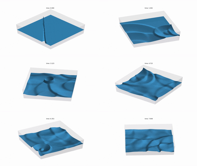
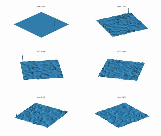
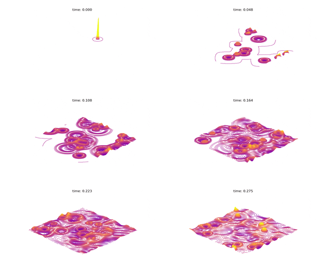
MattFlow simulates the surface of the water after any initial conditions, such as drops or stones falling on.
| requirements | os |
|---|---|
| python3 | GNU/Linux |
| click >= 7.0 | Windows |
| joblib >= 0.13.2 | OSX |
| matplotlib >= 3.3.1 | |
| numba >= 0.51.2 | |
| numpy >= 1.18.5 | |
| ffmpeg (optional) |
$ conda create --name mattflow -y
$ conda activate mattflow
$ conda install -c mattasa mattflow
$ pip install mattflow$ mattflow [OPTIONS]Options:
-m, --mode [drop|drops|rain] [default: drops]
-d, --drops INTEGER number of drops to generate [default: 5]
-s, --style [water|contour|wireframe]
[default: wireframe]
--rotation / --no-rotation rotate the domain [default: True]
-b, --basin render the fluid basin
--show / --no-show [default: True]
--save
--format [mp4|gif] [default: mp4]
--fps INTEGER [default: 18]
--dpi INTEGER [default: 75]
--fig-height INTEGER figure height (width is 1.618 * height)
[default: 18]
--help Show this message and exit.
SWE is a simplified CFD problem which models the surface of the water, with the assumption
that the horizontal length scale is much greater than the vertical length scale.
SWE is a coupled system of 3 hyperbolic partial differential equations, that derive from the
conservation of mass and the conservation of linear momentum (Navier-Stokes) equations, in
case of a horizontal stream bed, with no Coriolis, frictional or viscous forces (wiki).
where:
η : height
u : velocity along the x axis
υ : velocity along the y axis
ρ : density
g : gravity acceleration
- pre-process
structured/cartesian mesh - solution
supported solvers:- Lax-Friedrichs Riemann | O(Δt, Δx2, Δy2)
- 2-stage Runge-Kutta | O(Δt2, Δx2, Δy2) | default
- MacCormack | O(Δt2, Δx2, Δy2) | experimental
- post-processing
matplotlib animation
- mesh sizing
- domain sizing
- initial conditions (single drop, multiple drops, rain)
- boundary conditions (currently: reflective)
- solver
- multiprocessing
- plotting style
- animation options
- GUI
- Cython/C++
- Higher order schemes
- Source terms
- Viscous models
- Algorithm that converts every computational second to a real-time second,
modifying the fps at
the post-processing animation, because each iteration uses a different time-step (CFL condition). - Moving objects inside the domain
- 3D
GNU General Public License v3.0
Special thanks to Marios Mitalidis for the valuable feedback.
Start the flow!
(C) 2019, Athanasios Mattas
[email protected]


![{\displaystyle {\begin{aligned}{\frac {\partial (\rho \eta )}{\partial t}}&+{\frac {\partial (\rho \eta u)}{\partial x}}+{\frac {\partial (\rho \eta v)}{\partial y}}=0,\\[3pt]{\frac {\partial (\rho \eta u)}{\partial t}}&+{\frac {\partial }{\partial x}}\left(\rho \eta u^{2}+{\frac {1}{2}}\rho g\eta ^{2}\right)+{\frac {\partial (\rho \eta uv)}{\partial y}}=0,\\[3pt]{\frac {\partial (\rho \eta v)}{\partial t}}&+{\frac {\partial (\rho \eta uv)}{\partial x}}+{\frac {\partial }{\partial y}}\left(\rho \eta v^{2}+{\frac {1}{2}}\rho g\eta ^{2}\right)=0.\end{aligned}}}](https://wikimedia.org/api/rest_v1/media/math/render/svg/9b9d481407c0c835525291740de8d1c446265ce2)